**Transient Image Viewer**
The [Toolbox](/toolbox) contains a viewer that can be used to explore transient images.
Overview
========
The viewer implements two useful ways to display the three-dimensional datasets: The first one (called *Histogram view*) is a line plot where the dataset is integrated in the spatial dimension, thus showing the total amount of light that the reflector received at any point in time.
The second one (called *Time slice view*) shows a single time slice of the image, which visualises, where on the reflector the light was reflected at a certain time. Alternatively the image can be integrated in the temporal domain, resulting in a traditional (steady-state) camera image of the reflector.
In principle, the [transient image file format](/doc/transient-image-files) can store datasets with very little structure, but those are very hard to visualize in a generic way. Thus, the viewer currently supports only `Mode 10` where the reflector is sampled in a regular grid. This works well with all the data distributed in the benchmark, but may not be universal enough for transient images from different sources.
Download
========
The scripts are part of the toolbox and are available as a single [download](/toolbox).
Usage
========
The viewer is implemented in *Python* and *matplotlib* an can be easily adapted due to its relatively small size.
Histogram view
--------------
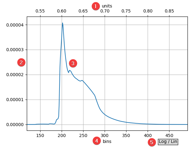
1. X-Axis in distance units. The plot has two different x-axes, one showing the distance in units (remember the synthetic data use arbitrary distance units) and one showing the associated time bins.
2. Y-Axis showing the average intensity per pixel at this time / distance.
3. The pixel intensities histogram plot. It can be manipulated using the standard matplotlib controls.
4. X-Axis in time bins. The plot has two different x-axes, one showing the distance in units (remember the synthetic data use arbitrary units) and one showing the associated time bins.
5. Log/Lin switch. Switches the y-axis from linear to logarithmic and back.
Time slice view
---------------
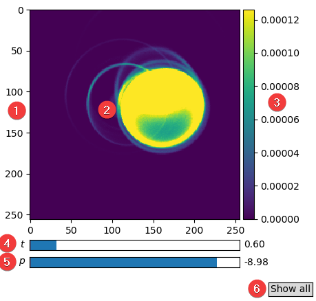
1. X and Y axis in pixels. This pixels are displayed as they appear on the camera sensor not as they appear on the reflector (this transformation is given through the 4 corner points in the transient image file, however all benchmark data use a orthographic projection).
2. The actual plot. It can be manipulated using the standard matplotlib controls.
3. The colorbar and associated data range.
4. Slider for the time slice to be displayed. On the right, the distance in units of the current time slice is shown.
5. Intensity slider used to adjust the colorbar range. Due to the high dynamic range, it is difficult to display all details of a single slice in a static picture. On the right side, the exponent resulting in the scale factor is shown. (The actual meanings of the colors can be seen in the colorbar, however this number is useful to quickly set two independent plots to the same intensity.)
6. `Show all` button to switch on temporal integration. In this mode, received light from any time is shown. To switch back to single slice view, select a time slice with the time slice slider (4.).
Advanced usage
==============
These tools help to get a quick overview of transient images. Instead of providing a complex UI for more advanced plots, we encourage users to use matplotlib directly with the loaded data to write their own plots. This can usually be done in very few lines and offers a flexibility that could not be provided by a UI.